本文基于定制化的TFLite Micro动态链接库,通过”hello world”示例来验证TFLite Micro版本的功能。虽然名字叫是”hello world”,其实并不是在控制台上打印出”hello world”这么简单,而是用Python版本的Tensorflow构建训练一个能够学习并生成正弦波的模型,通过TFLite的转换器转换为.tflite文件,并使用TFLite Micro动态链接库加载并执行推断的过程
开发环境
Inter i5-7200U
Ubuntu18.04.2 x86_64
conda Python3.7虚拟环境
Tensorflow2.1.0
参考
tensorflow/tensorflow/lite/micro/examples/hello_world/create_sine_model.ipynb
生成数据
首先需要加载一些python库
1 | import tensorflow as tf |
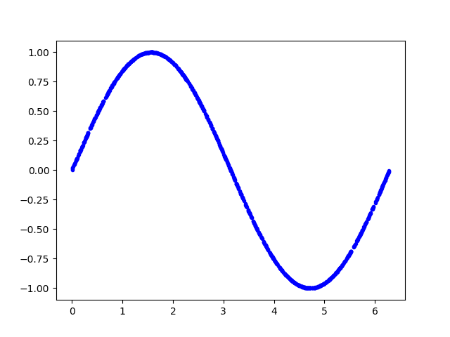
以下代码生成一组随机数,并计算它们的正弦值,并绘图显示
1 | SAMPLES = 1000 |
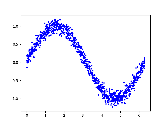
添加噪声
由于数据是由正弦函数直接生成,数据太过平滑。然而现实中获取的各种信号必然夹杂着噪声数据,而机器学习算法能够从带有噪声的数据中学习到真正的信息
为数据添加一些噪声,并绘制显示
1 | y_values += 0.1 * np.random.randn(*y_values.shape) |
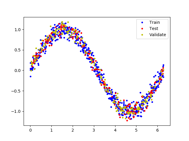
拆分数据
我们已经生成了一个近似真实世界的噪声数据,我们用它来训练模型
为了验证评估模型,以及防止数据的过拟合,我们将数据拆分为训练集、测试集和验证集3部分,比例为3:1:1
以下代码将数据分割,并以不同的颜色显示
1 | TRAIN_SPLIT = int(0.6 * SAMPLES) |
设计模型
我们将建立一个模型,它接收一个输入,并用它来预测一个输出,此类问题称为回归问题。为了达到这个目的,我们将创建一个简单的神经网络,它将使用多层的神经元来学习数据背后的模式,以便进行预测
首先,我们定义两个层。第一层接收一个输入,并经过16个神经元。输入到来时,每个神经元将根据自身的权重和偏置状态受到不同程度的激活,神经元的激活程度由数字表示。第一层的激活将作为第二层的输入,第二层的输出作为模型的输出值
我们使用Keras来定义模型,模型使用”relu”作为激活函数,优化器使用”rmsprop”,损失函数使用”mse”,使用MAE来评估
1 | from tensorflow.keras import layers |
训练模型
一旦我们定义好了模型,可以使用数据来训练它。训练过程将x输入到网络中,检查网络输出与原始数据的偏离程度,并调整神经元的偏置和权重。训练过程是在整个数据上多次运行,每次完整的运行都称为”epoch”。在每个”epoch”中,数据以多批次的方式在网络中运行,每一批次都有几个数据进入网络并输出,对网络参数的调整是以一个批次为单位的。”epoch”次数和批次大小都可以通过参数调整
以下代码运行1000个”epoch”,每个批次16个数据,还传递一些数据用于验证。整个训练需要一定的时间
1 | history_1 = model_1.fit(x_train, y_train, epochs=1000, batch_size=16, |
模型评估
在训练期间,模型的性能在数据迭代中不断的提升,训练会生成一个日志,告诉我们性能在训练过程中是如何变化的。以下代码将以图形形式显示其中一些信息
1 | loss = history_1.history['loss'] |
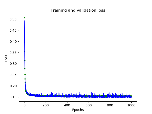
图形中显示了每个epoch的损失函数情况。有多种方式的损失函数,这里我们使用的是均方误差MSE。损失函数在前25个epoch迅速减少,之后趋于平缓,这意味着模型在不断改进。我们的目标是当模型不再改进,或者当训练损失小于验证损失时,意味着学习已经收敛,需要停止训练。为了更清楚的观察平坦部分,我们跳过前50个epoch的训练情况
1 | SKIP = 50 |
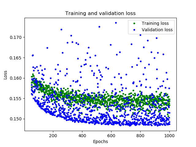
从上图中可以看出,损失在前600个epoch持续减少,到600之后不再变化,这意味着600之后的训练是没有必要的。同时,我们也可以看到,最低的损失函数值仍然在0.155左右,这意味着我们的网络预测平均偏离了15%。另外,验证损失值跳变很多。为了了解更多模型的性能,我们可以绘制更多数据,这次我们输出MAE平均绝对误差,这是测量网络预测与实际之间差距距离的另一种方法
1 | plt.clf() |
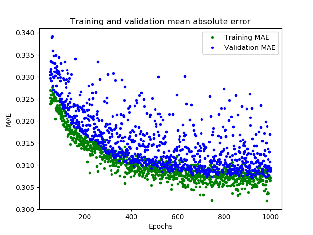
这幅图告诉了我们更多的信息。训练数据的MAE始终低于验证数据的MAE,这意味着网络可能有过拟合,或者学习训练数据太僵硬,以至于无法对新数据做出有效预测。此外,MAE整体都较高,最多为0.305,这表明模型的预测有30%的偏差。为了更清楚的了解到发生了什么,我们可以将网络预测值和实际训练值进行比较
1 | predictions = model_1.predict(x_train) |
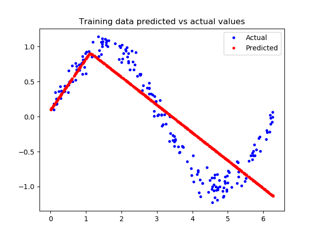
这张图表明网络已经学会以非常有限的方式逼近正弦函数,但是这是一个线性的逼近。这种拟合的刚性表明,该模型没有足够的能力来学习正弦波函数的全部复杂性,因此只能用过于简单的方法来近似它。我们可以修改模型,来改进性能
改变模型
再增加一层神经元,以下增加一个16个神经元的层
1 | model_2 = tf.keras.Sequential() |
我们现在将训练新模型。为了节省时间,我们只训练600个epoch
1 | history_2 = model_2.fit(x_train, y_train, epochs=600, batch_size=16, |
再次评估模型
可以看到,模型已经有了很大改进,验证损失从0.15降到0.015,验证MAE从0.31降低到0.1
以下代码显示新模型训练的情况
1 | loss = history_2.history['loss'] |
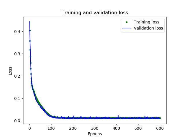
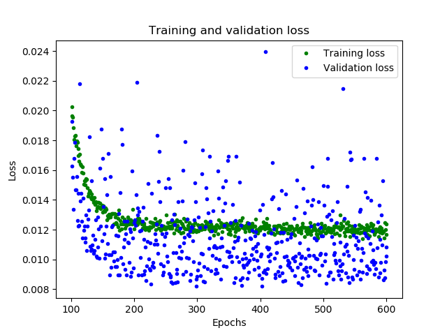
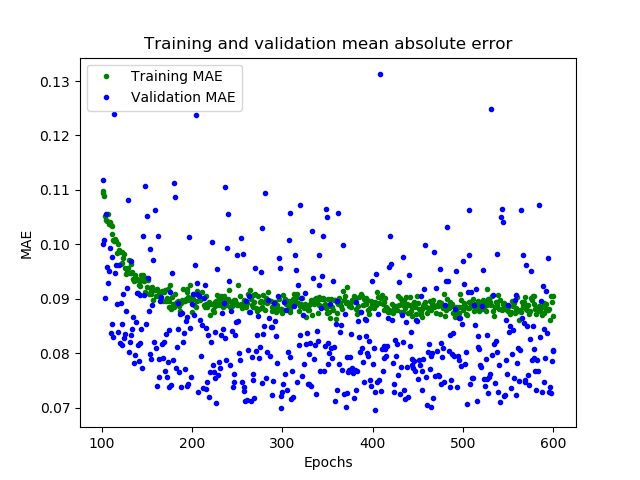
很好的结果,从图中可以看到一些令人兴奋的事情
我们的网络已经更快地达到了它的最高精度(在200个epoch而不是600个)
总的损失和MAE比之前的网络好得多
验证误差比训练误差更小,这意味着网络并没有过拟合
让我们对照模型的预测值和训练数据
1 | loss = model_2.evaluate(x_test, y_test) |
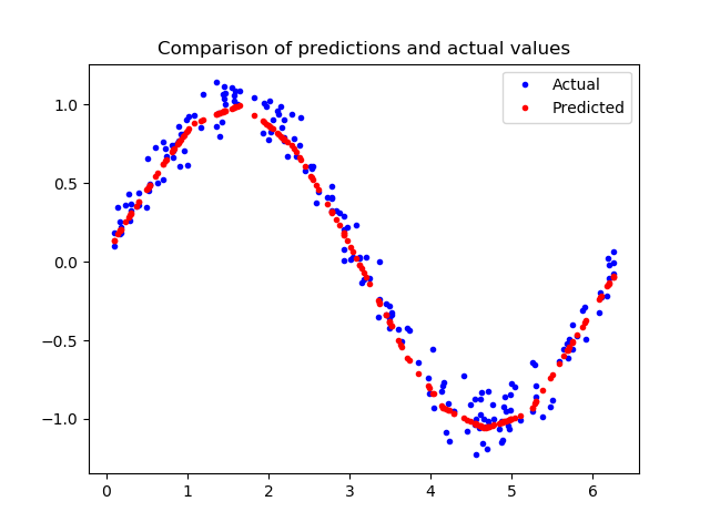
由上图看出,预测结果与我们的数据非常吻合。这个模型并不完美,它的预测并没有形成一个平滑的正弦曲线,如果我们想更进一步,我们可以尝试进一步增加模型的容量,也许可以使用一些技术来防止过度拟合。然而,机器学习的一个重要部分是知道什么时候停止,这个模型对于我们示例来说已经足够好了
转换模型到TFLite
将模型用于TFLite微控制器,需要将其转换为正确的格式,为此我们将使用Tensorflow Lite转换器,转换器可以以一种特殊的、节省空间的格式将模型输出到文件。由于是部署到微控制器上,我们希望它尽可能小,可以通过量化的方法减小尺寸。它降低了模型权重的精度,以节省内存。因为量化模型更小,因此运行起来也更快
转换器可以在转换时选择是否进行量化
1 | converter = tf.lite.TFLiteConverter.from_keras_model(model_2) |
执行以上代码可以看到,未量化的模型大小为2732KB,量化模型大小为2720KB
测试转换后的模型
为了证明这些模型在转换和量化之后仍然是准确的,我们将使用这两个模型进行预测,并将其与我们的测试结果进行比较:
1 | sine_model = tf.lite.Interpreter('sine_model.tflite') |
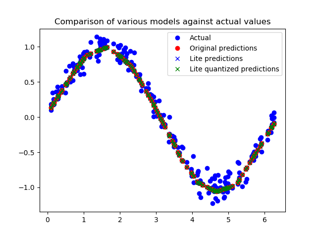
从图中我们可以看出,对原始模型、转换模型和量化模型的预测都非常接近,无法区分。这意味着我们的量化模型已经可以使用了!
使用C++程序执行推断
这里使用C++程序需要依赖TFLite Micro动态链接库,参见
通过xxd命令将模型文件转换为C++源文件
1 | xxd -i sine_model_quantized.tflite > sine_model_quantized.cc |
可以看到生成的C++文件中,模型是以字节序列存放的,并通过sine_model_quantized.h文件向外暴露模型地址和长度
1 | unsigned char sine_model_quantized_tflite[] = { |
我们创建一个main.cc源文件,用来加载模型并循环执行推断,将模型输出导出到csv文件中,最后用python绘图呈现模型的预测效果
引用一些头文件
TFLite Micro程序需要引用一些必要的头文件
1 |
|
all_ops_resolver.h文件中定义了一些优化器相关的运算组建,例如全连接(Full Connected, FC)、柔性最大化函数Softmax、卷积conv
micro_error_reporter.h文件中定义了调试方法
micro_interpreter.h文件中是解释器的定义
sin_model_data.h引用模型文件
加载模型
首先创建一个调试器reporter
1 | tflite::MicroErrorReporter micro_error_reporter; |
调用GetModel()方法加载模型
1 | const tflite::Model* model = ::tflite::GetModel(g_sine_model_data); |
创建一个运算器
1 | tflite::ops::micro::AllOpsResolver resolver; |
创建解释器,并为模型推断分配内存空间
1 | const int tensor_arena_size = 10 * 1024; |
创建指针指向模型输入和输出
1 | tflite::MicroInterpreter *inter = &interpreter; |
创建csv文件”data.csv”
1 | ofstream outFile; |
以下循环,产生1000个输入,执行模型推断,并将输入和输出保存到csv文件,并打印到屏幕
1 | int kInferencesPerCycle = 1000; |
运行结果
编译程序并运行,数据保存到了”data.csv”文件中,查看其内容
1 | cat data.csv | head -n 20 |
编写python脚本draw.py读取data.csv文件并将数值绘制出来
1 | import matplotlib.pyplot as plt |
执行脚本
1 | python draw.py |
结果如图
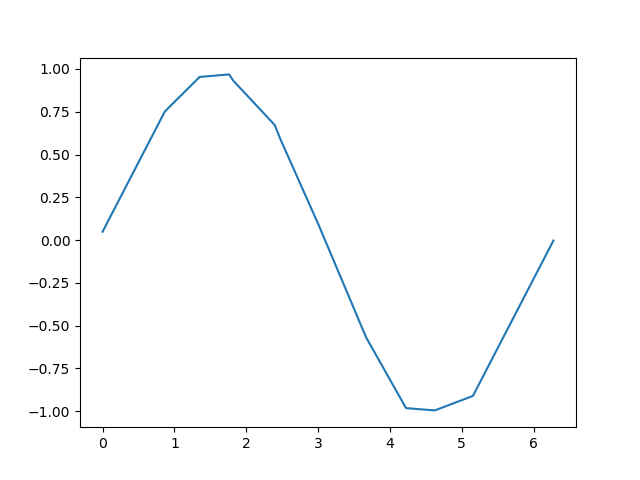
可见模型输出的结果准确