DIP-高斯滤波器

简单的盒式滤波器有很多局限性,在涉及精细细节或者强几何分量的应用中,并不适用。高斯滤波器相比盒式滤波器更有优势
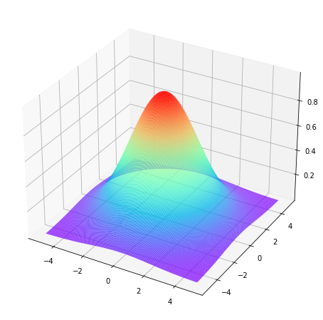
高斯核定义如下

\begin{equation}
w(s,t)=Ke^{-\frac{s^{2} + t^{2}}{2 \sigma^{2}}}
\end{equation}

高斯核是唯一可分离的圆对称核

可分离性

如果二维函数$G(x,y)$可表示为两个一维函数的乘积$G{1}(x)G{2}(x)$,则称它是可分离的。对于空间滤波器而言,可分离的核能够表示为两个向量的外积

\begin{equation}
w = uv^{T}
\end{equation}

由于卷积满足交换律和结合律,可分离性可以带来卷积运算复杂度上的降低。假设图像$f$大小为$m \times n$,卷积核$w$大小为$a \times b$,如果按照正常的卷积运算,需要$mnab$次卷积运算。如果卷积核为可分离的,那么可将$w$分离为$w{1}$和$w{2}$,$f \ast w$可拆分为$f \ast w{1} \ast w{2}$,和$w{1}$的运算需要$mna$次卷积,其结果和$w{2}$运算需要$mnb$次卷积,因此可分离核卷积与不可分离核卷积运算量比为

\begin{equation}
C = \frac{mn(a+b)}{mnab} = \frac{a+b}{ab}
\end{equation}

判断一个滤波器是否为可分离的,只需确定其秩是否为1,如果为1,表明是可分离的

圆对称性

圆对称性也叫做各向同性,即其响应与方向无关,这意味着卷积操作不会带来方向性的负面效果。

以下仿真产生一个$5 \times 5, K=1, \sigma=1$的高斯核

1
2
3
4
5
6
7
8
9
10
11
12
import numpy as np

def gaussian_kernel(x, y, k, sigma):
return k * np.exp(-(x**2+y**2)/(2*sigma**2))

kernel = np.zeros((11, 11))
for i in range(kernel.shape[0]):
for j in range(kernel.shape[1]):
x = np.abs(i-5)
y = np.abs(j-5)
kernel[i, j] = round(gaussian_kernel(x, y, 1, 1), 3)
print(kernel)
1
2
3
4
5
6
7
8
9
10
11
[[0.    0.    0.    0.    0.    0.    0.    0.    0.    0.    0.   ]
[0. 0. 0. 0. 0. 0. 0. 0. 0. 0. 0. ]
[0. 0. 0. 0.002 0.007 0.011 0.007 0.002 0. 0. 0. ]
[0. 0. 0.002 0.018 0.082 0.135 0.082 0.018 0.002 0. 0. ]
[0. 0. 0.007 0.082 0.368 0.607 0.368 0.082 0.007 0. 0. ]
[0. 0. 0.011 0.135 0.607 1. 0.607 0.135 0.011 0. 0. ]
[0. 0. 0.007 0.082 0.368 0.607 0.368 0.082 0.007 0. 0. ]
[0. 0. 0.002 0.018 0.082 0.135 0.082 0.018 0.002 0. 0. ]
[0. 0. 0. 0.002 0.007 0.011 0.007 0.002 0. 0. 0. ]
[0. 0. 0. 0. 0. 0. 0. 0. 0. 0. 0. ]
[0. 0. 0. 0. 0. 0. 0. 0. 0. 0. 0. ]]

可以看到,核中心值为1,与中心距离相同的位置值相同

3$\sigma$

高斯函数的性质存在一个3倍$\sigma$位置,距均值距离超过$3\sigma$的点数值上非常小,如果选择高斯核大小为$6\sigma \times 6 \sigma$,那么得到的结果与使用任意比其大的高斯核处理结果相同。因此,如果$\sigma=7$,则应使用$43 \times 43$的高斯核

高斯函数的乘积和卷积仍是高斯函数

贝叶斯估计就是源于此,两个高斯分布相乘仍是高斯分布,新的高斯分布方差更小,均值更大

因此,多个高斯核的卷积处理可以合并为1个高斯核的卷积

两个高斯核卷积后的均值等于两个均值的和,由于用高斯做卷积时均值为0,因此均值项可以不考虑

\begin{equation}
m{f \ast g}=m{f} + m_{g}
\end{equation}

卷积前后方差的关系为

\begin{equation}
\sigma{f \ast g} = \sqrt{\sigma{f}^{2}+ \sigma_{g}^{2}}
\end{equation}

如果多个高斯核的大小都是$m \times m$,则合并的核大小$W \times W$为

\begin{equation}
W = Q \times (m-1 + m)
\end{equation}

其中Q为高斯核数量

Python Code

1
2
3
4
5
6
7
8
9
10
11
12
13
14
15
16
17
18
19
20
21
22
23
24
25
26
27
28
29
30
31
32
33
34
35
36
import matplotlib.pyplot as plt
import numpy as np
import cv2 as cv

def conv2d_kernel(matrix, kernel):
n = len(kernel)
ans = 0
for i in range(n):
for j in range(n):
ans += matrix[i,j]*float(kernel[i,j])
return ans

def image_conv2d(im, kernel):
n = len(kernel)
# padding size: 2*(kernelsize - 1)
im_padding = np.zeros((im.shape[0]+2*(n-1), im.shape[1]+2*(n-1)))
# im data copy to padding matrix
im_padding[(n-1):(n+im.shape[0]-1), (n-1):(n+im.shape[1]-1)] = im
im_conv = np.zeros((im_padding.shape[0]-n+1, im_padding.shape[1]-n+1))
for i in range(im_padding.shape[0]-n+1):
for j in range(im_padding.shape[1]-n+1):
neighbor = im_padding[i:i+n, j:j+n]
im_conv[i, j] = conv2d_kernel(neighbor, kernel)
pos = int((n-1)/2)
im_new = im_conv[pos:(pos+im.shape[0]), pos:(pos+im.shape[1])]
return im_new

def gaussian_kernel_create(size, k, sigma):
kernel = np.zeros((size, size))
center = (size-1)/2
for i in range(kernel.shape[0]):
for j in range(kernel.shape[1]):
x = np.abs(i-center)
y = np.abs(j-center)
kernel[i, j] = k * np.exp(-(x**2+y**2)/(2*sigma**2))
return kernel/np.sum(kernel)

分别以$7 \times 7, \sigma=1$和$21 \times 21, \sigma=3.5$创建两个高斯核

1
2
kernel_1 = gaussian_kernel_create(7, 1, 1)
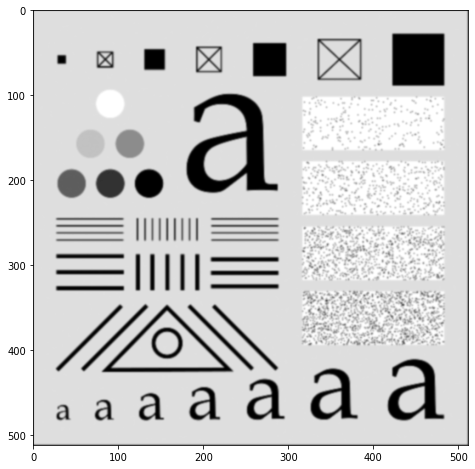
kernel_2 = gaussian_kernel_create(21, 1, 3.5)

显示原始图像

1
2
aussian_kernel_create(21, 1, 3.5)
im = cv.imread('images/02.tif', 0)

$7 \times 7$卷积核处理后的图像

1
2
im_out1 = image_conv2d(im, kernel_1)
plt.imshow(im_out1, cmap='gray')

$21 \times 21$卷积核处理后的图像

1
2
im_out2 = image_conv2d(im, kernel_2)
plt.imshow(im_out2, cmap='gray')

以$21\times 21, \sigma=1$创建高斯核,可以看到处理结果与$7 \times 7, \sigma=1$处理结果基本一致

1
2
3
kernel_3 = gaussian_kernel_create(21, 1, 1)
im_out3 = image_conv2d(im, kernel_3)
plt.imshow(im_out3, cmap='gray')