图像金字塔对于执行多尺度的编辑操作非常有效,能够在保持图像细节的同时进行融合。Peter J. Burt等人在1983年的”The Laplacian Pyramid as a Compact Image Code”中提出了拉普拉斯金字塔用于图像压缩,后来该方法被用于图像融合效果很好
本文首先对拉普拉斯金字塔进行介绍,然后对拉普拉斯用于图像融合进行介绍
Laplacian Pyramid
拉普拉斯金字塔通过将原始图像减去一个低通滤波的图像来消除像素间的相关性,得到一个净数据压缩,仅保留了差异。将这种做法在多尺度上进行迭代,会得到一个这种差异的金字塔,由于这种做法相当于用拉普拉斯算子对图像进行多尺度采样,因此得到的金字塔叫做拉普拉斯金字塔
该方法用于数据压缩时,仅需保留金字塔最小分辨率(最低层次)的低通图像以及一个拉普拉斯金字塔,就可以完全恢复原始图像。在重建原始图像时,将最小分辨率的低通图像逐层与拉普拉斯金字塔进行结合,最终获得压缩前的原始图像
下图是整个拉普拉斯金字塔的构建和重建原始图像的示意图
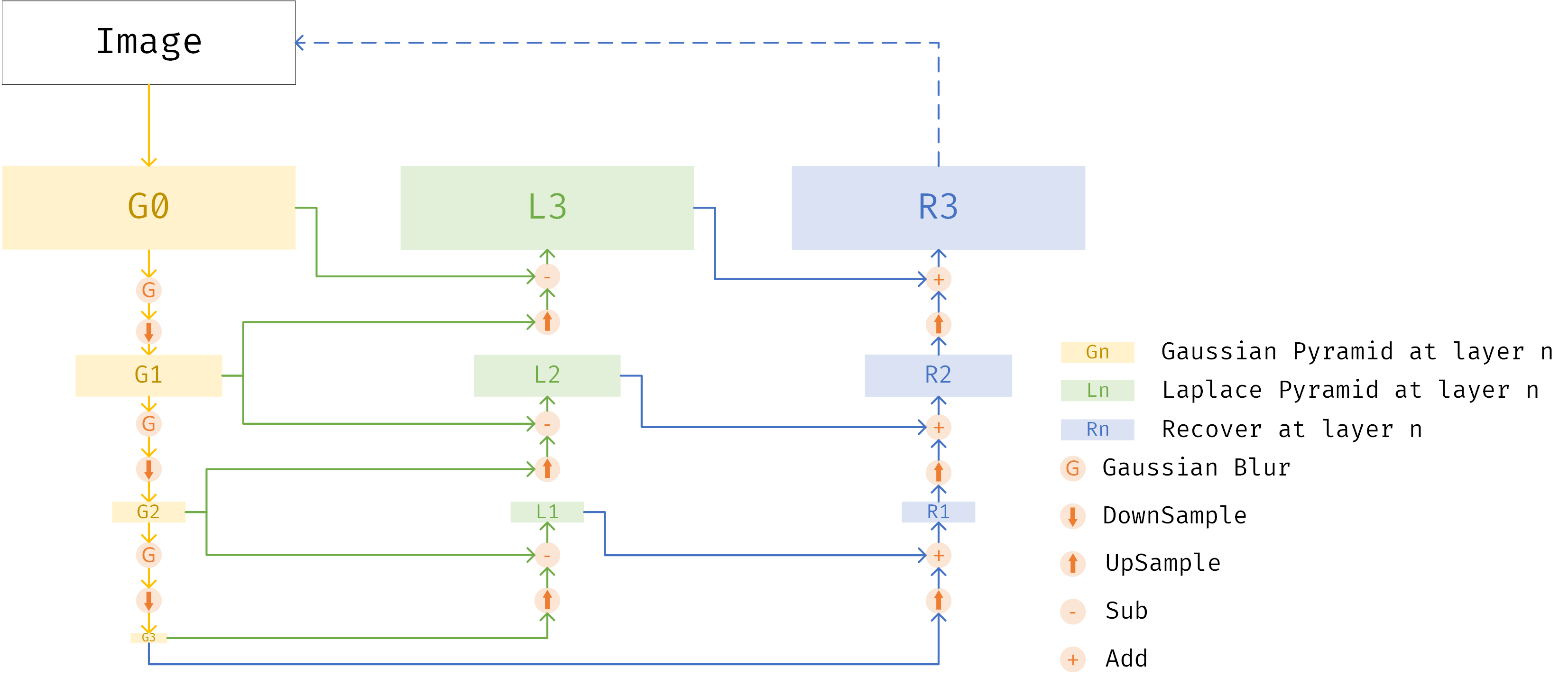
该过程中主要涉及到以下几种处理
高斯滤波或高斯模糊(Gaussian Blur)
上采样(UpSample)
下采样(DownSample)
图像相加和相减
高斯滤波主要关注核大小与方差,下采样比较好做,按偶数或奇数行采样即可。上采样可以使用各种插值方法如三次样条插值等
拉普拉斯金字塔的生成
拉普拉斯金字塔的生成需要依赖高斯金字塔,上图中的黄色部分是生成高斯金字塔的过程。”Image”表示原始图像,以3层金字塔为例,G0即原始图像,经过高斯滤波和下采样得到尺度缩小为1/4的低通图像G1,重复该过程得到G2、G3,[G0, G1, G2, G3]构成了4层的高斯金字塔
拉普拉斯金字塔的每层由对应层的高斯金字塔图像与高斯金字塔下层图像的上采样相减得到,例如L3是由1/4原始尺度的G1经过上采样,在与G0相减得到。L2是由G2上采样与G1相减得到。实际需要使用的拉普拉斯金字塔只有3层,即[L1, L2, L3]
python代码如下
导入库
1 | import cv2 |
定义高斯金字塔生成函数
1 | def gaussian_pyramid(im, layers): |
定义拉普拉斯金字塔生成函数
1 | def laplace_pyramid(im, layers): |
定义金字塔信息打印与显示函数
1 | cv2.namedWindow('img', cv2.WINDOW_NORMAL) |
读入图像生成4层的高斯金字塔并显示
1 | im = cv2.imread('images/cat.jpeg') |
1 | ---- GPyrs's info ---- |
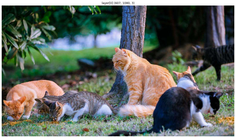
G0层图像
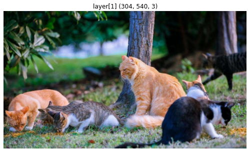
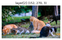
G1层图像
G2层图像
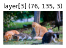
G3层图像
生成4层拉普拉斯金字塔并显示
1 | LPyrs = laplace_pyramid(im, 4) |
1 | ---- LPyrs's info ---- |
L0层图像

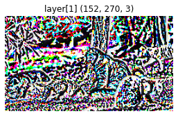
L1层图像
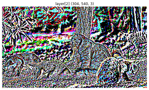
L2层图像
L3层图像
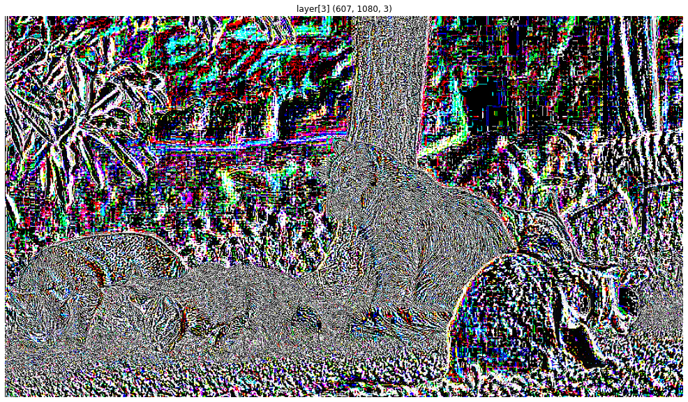
可以看到拉普拉斯图像中的每幅图像主要是纹理特征
原始图像重建
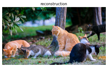
重建过程由最小分辨率开始的低通图像开始,经过上采样并与拉普莱斯金字塔对应分辨率图像相加,并经过多次向上迭代,最终得到原始图像并显示
1 | reconstruction = LPyrs[0] |
结果如下图,能够正常复原原始图像
图像融合
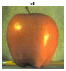
利用拉普拉斯金字塔进行图像融合是一个非常有趣的应用。融合后的图像在交界处的变化是非常平滑的,图像上的高频纹理混合得更快,可以避免 “鬼影”效果。为了创建融合图像,每幅图像首先生成自己的拉普拉斯金字塔,然后用一个二值掩模图像生成的高斯金字塔作为融合的权重金字塔,与两幅待融合的拉普拉斯金字塔进行结合,得到融合后的拉普拉斯金字塔,最后用融合后的拉普拉斯金字塔与最小分辨率的融合低通图像进行重建,最终得到融合的图像
加载左右两幅待融合图像以及二值掩模图像并显示
1 | layers = 7 |
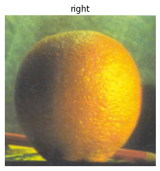
显示右图
1 | plt.axis('off') |
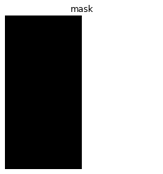
显示二值掩模图像
1 | plt.axis('off') |
图像预处理
1 | # 大小调整为256x256 |
计算left、right、mask的高斯金字塔,left和right的拉普拉斯金字塔
1 | # 生成高斯金字塔 |
打印各金字塔尺度
1 | layers_info_print(left_G, 'right_G') |
1 | ---- left_G's info ---- |
生成融合拉普拉斯金字塔
1 | blend_L = [] |
1 | ---- blend_L's info ---- |
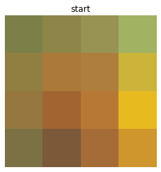
计算最小分辨率低通融合图像
1 | start = (mask_G_r[-1])*left_G[-1] + (mask_G[-1])*right_G[-1] |
进行融合
1 | blend = start |
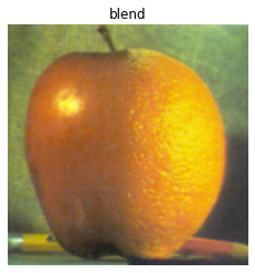
最终融合后的图像如下