VitisAI-07-模型部署

本文以自定义模型为例,对使用VitisAI进行模型量化部署的流程进行介绍

Workflow

  • 数据集为fashion_mnist

  • 使用Tensorflow2搭建一个简单分类网络并进行训练,导出模型文件

  • 使用VitsiAI docker中的vai_q_tensorflow2工具进行模型量化和校准,得到校准模型文件

  • 使用VitisAI docker中的vai_c_tensorflow2工具进行模型编译,生成能够部署在DPU上的模型文件

  • 编写模型推理程序(Python),并将推理程序、编译后的模型文件以及测试图片导入设备中,运行推理程序进行图片分类

Train

keras内置了fashion_mnist数据集,该数据集是小尺寸商品分类数据集,由28x28的单通道灰度图构成,训练集为60000张图片,测试集为10000张图片

导入包并加载数据集

1
2
3
4
5
6
7
8
9
import cv2 as cv
import numpy as np
from PIL import Image
import tensorflow as tf
from tensorflow import keras
import matplotlib.pyplot as plt

fashion_mnist = keras.datasets.fashion_mnist
(train_images, train_labels), (test_images, test_labels) = fashion_mnist.load_data()

查看数据集

1
2
print(train_images.shape)
print(test_images.shape)
1
2
(60000, 28, 28)
(10000, 28, 28)

保存一些测试数据为图片

1
2
3
4
5
def test_image_save(images, num=32):
for i in range(num):
img = Image.fromarray(images[i])
img.save('images/{}.jpg'.format(i), quality=100)
test_image_save(test_images, num=32)

构建模型并打印summary

1
2
3
4
5
6
7
8
9
10
11
12
13
train_images = train_images.reshape((60000, 28,28,1))
test_images = test_images.reshape((10000, 28,28,1))
np.save('train_images', train_images)
np.save('test_images', test_images)
np.save('test_labels', test_labels)
model = keras.Sequential([
keras.layers.Conv2D(16, (3,3), activation='relu',
input_shape=(28,28,1)),
keras.layers.Flatten(),
keras.layers.Dense(128, activation='relu'),
keras.layers.Dense(10)
])
model.summary()
1
2
3
4
5
6
7
8
9
10
11
12
13
14
15
16
Model: "sequential"
_________________________________________________________________
Layer (type) Output Shape Param #
=================================================================
conv2d (Conv2D) (None, 26, 26, 16) 160
_________________________________________________________________
flatten (Flatten) (None, 10816) 0
_________________________________________________________________
dense (Dense) (None, 128) 1384576
_________________________________________________________________
dense_1 (Dense) (None, 10) 1290
=================================================================
Total params: 1,386,026
Trainable params: 1,386,026
Non-trainable params: 0
_________________________________________________________________

编译并训练模型

1
2
3
4
model.compile(optimizer='adam',
loss=tf.keras.losses.SparseCategoricalCrossentropy(from_logits=True),
metrics=['accuracy'])
model.fit(train_images, train_labels, epochs=10)
1
2
3
4
5
6
7
8
9
10
11
12
13
14
15
16
17
18
19
20
21
22
23
24
25
26
27
28
29
30
Epoch 1/20
1875/1875 [==============================] - 13s 7ms/step - loss: 1.9238 - accuracy: 0.8173
Epoch 2/20
1875/1875 [==============================] - 13s 7ms/step - loss: 0.3347 - accuracy: 0.8827
Epoch 3/20
1875/1875 [==============================] - 13s 7ms/step - loss: 0.2755 - accuracy: 0.8995
Epoch 4/20
1875/1875 [==============================] - 13s 7ms/step - loss: 0.2399 - accuracy: 0.9123 0s -
Epoch 5/20
1875/1875 [==============================] - 14s 7ms/step - loss: 0.2122 - accuracy: 0.9227
Epoch 6/20
1875/1875 [==============================] - 13s 7ms/step - loss: 0.1852 - accuracy: 0.9323 0s -
Epoch 7/20
1875/1875 [==============================] - 13s 7ms/step - loss: 0.1617 - accuracy: 0.9408
Epoch 8/20
1875/1875 [==============================] - 13s 7ms/step - loss: 0.1429 - accuracy: 0.9478
Epoch 9/20
1875/1875 [==============================] - 13s 7ms/step - loss: 0.1321 - accuracy: 0.9518
Epoch 10/20
1875/1875 [==============================] - 13s 7ms/step - loss: 0.1153 - accuracy: 0.9586
Epoch 11/20
1875/1875 [==============================] - 13s 7ms/step - loss: 0.1039 - accuracy: 0.9626
Epoch 12/20
1875/1875 [==============================] - 13s 7ms/step - loss: 0.0935 - accuracy: 0.9658
Epoch 13/20
...
Epoch 19/20
1875/1875 [==============================] - 13s 7ms/step - loss: 0.0579 - accuracy: 0.9800
Epoch 20/20
1875/1875 [==============================] - 13s 7ms/step - loss: 0.0550 - accuracy: 0.9805

在测试集验证精度并保存模型为.h5文件

1
2
3
test_loss, test_acc = model.evaluate(test_images,  test_labels, verbose=2)
print('\nTest accuracy:', test_acc)
model.save('tf2_fmnist_model.h5')

精度还可以吧,毕竟只是随便搭个模型验证流程用的

1
2
313/313 - 1s - loss: 1.0434 - accuracy: 0.8792
Test accuracy: 0.8791999816894531

Quantization and Compile

VitisAI的量化和编译工具在docker中。VAI(VitisAi)量化器以一个浮点模型作为输入,这个浮点模型可以是Tensorflow1.x/2.x、Caffe或者PyTorch生成的模型文件,在量化器中会进行一些预处理,例如折叠BN、删除不需要的节点等,然后对权重、偏置和激活函数量化到指定的位宽(目前仅支持INT8)
为了抓取激活函数的统计信息并提高量化模型的准确性,VAI量化器必须运行多次推理来进行校准。校准需要一个100~1000个样本的数据作为输入,这个过程只需要unlabel的图片就可以
校准完成后生成量化过的定点模型,该模型还必须经过编译,以生成可以部署在DPU上的模型

Quantization the model

由于训练模型使用的是Tensorflow2,因此这里必须使用docker的vai_q_tensorflow2来进行量化,读者如果使用的是其他框架,请使用对应的量化工具。请注意这里的vai_q_tensorflow2等量化工具并非是Tensorflow提供的,而是VitisAI为不同的深度学习框架定制的量化工具,请勿混淆

VitisAI中共支持以下4种量化方式

  • vai_q_tensorflow:用于量化Tensorflow1.x训练的模型
  • vai_q_tensorflow2:用于量化Tensorflow2.x训练的模型
  • vai_q_pytorch:用于量化Pytorch训练的模型
  • vai_q_caffe:用于量化caffe训练的模型

这四种量化工具都在docker中,但是在不同的conda虚拟环境中,因此启动进入docker后需要先激活对应的conda环境

1
2
./docker_run.sh xilinx/vitis-ai
conda activate vitis-ai-tensorflow2

vai_q_tensorflow2支持两种不同的方法来量化模型

  • Post-training quantization (PTQ):PTQ是一种将预先训练好的浮点模型转换为量化模型的技术,模型精度几乎没有降低。需要一个具有代表性的数据集对浮点模型进行batch推断,以获得激活函数的分布。这个过程也叫量化校准
  • Quantization aware training(QAT):QAT在模型量化期间对前向和后向过程中的量化误差进行建模,对于QAT,建议从精度良好的浮点预训练模型开始,而不是从头开始

本文选用的是PTQ方式。在VitisAI/models路径下创建文件夹mymodel,将以下文件放入其中

  • 训练生成的tf2_fmnist_model.h5文件
  • 训练集train_images.npy用于校准
  • 测试集test_images.npy、测试标签test_labels用于校准后的评估

编写quantization.py量化脚本

1
2
3
4
5
6
7
8
9
10
11
12
13
14
15
16
17
18
19
20
21
22
23
24
25
26
27
28
29
30
31
32
33
34
35
36
37
import os
import numpy as np
import tensorflow as tf
from tensorflow import keras
from tensorflow_model_optimization.quantization.keras import vitis_quantize

train_images = np.load('train_images.npy')
test_images = np.load('test_images.npy')
test_labels = np.load('test_labels.npy')

# load float model
float_model = tf.keras.models.load_model('tf2_fmnist_model.h5')

quantizer = vitis_quantize.VitisQuantizer(float_model)

# Set calibration dataset to train_images, save quantized model to quantized.h5
quantized_model = quantizer.quantize_model(
calib_dataset=train_images[0:10],
include_cle=True,
cle_steps=10,
include_fast_ft=True
)
quantized_model.save('quantized.h5')

# Load quantized model
quantized_model = keras.models.load_model('quantized.h5')

# Evaluate quantized model
quantized_model.compile(
loss=tf.keras.losses.SparseCategoricalCrossentropy(from_logits=True),
metrics=['sparse_categorical_accuracy']
)
quantized_model.evaluate(test_images, test_labels, batch_size=500)

# Dump quantized model
quantizer.dump_model(
quantized_model, dataset=train_images[0:1], dump_float=True)

运行该脚本

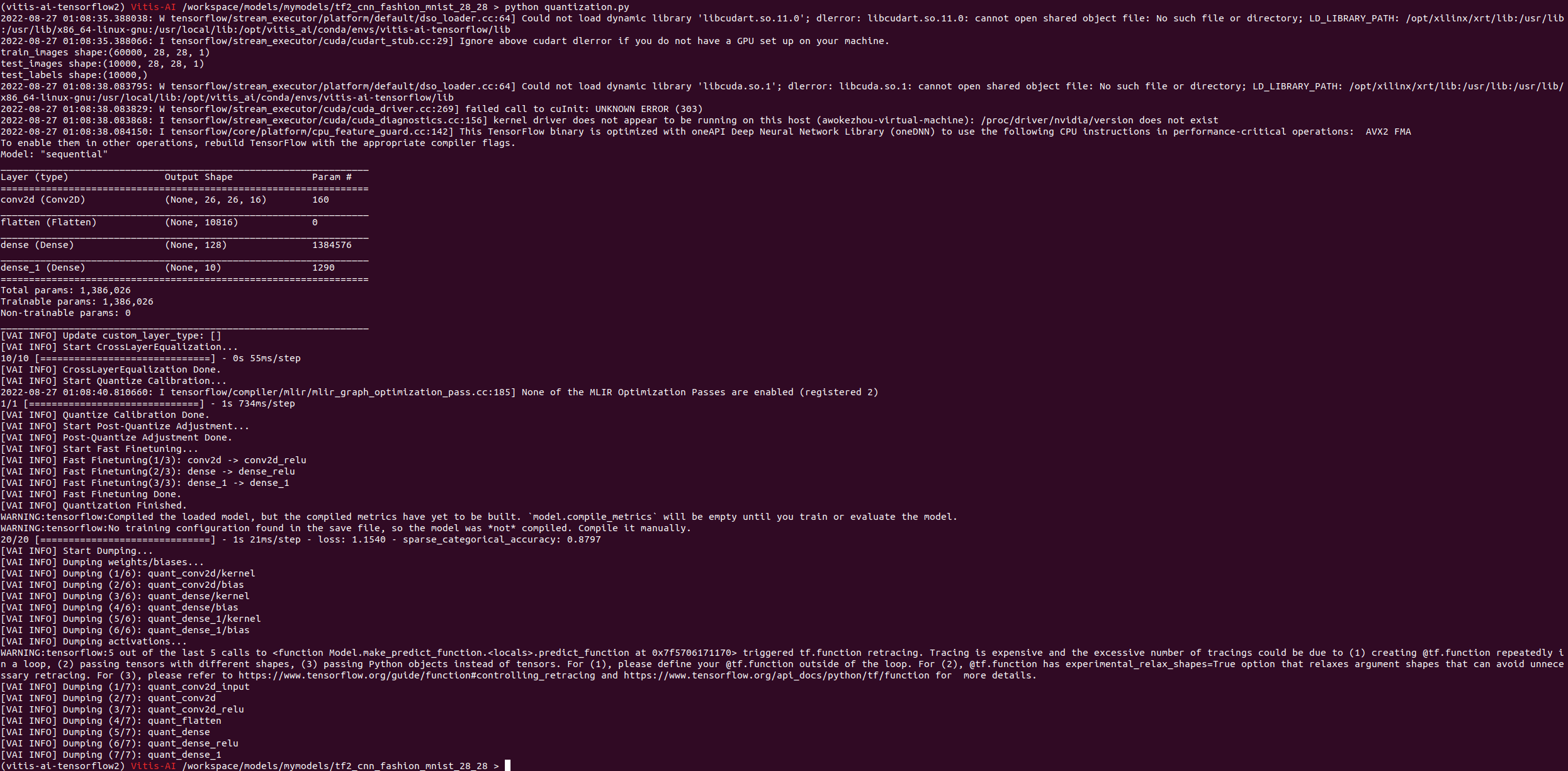
在目录下生成了quantized.h5量化模型文件,可以看到量化后的模型在测试集上评估精度为0.8797

Compile the model

编译模型需要准备以下文件

  • quantized.h5:量化生成的模型文件

  • arch.json:DPU描述文件,在vitis项目中,dpu_trd_system_hw_link/Hardware/dpu.build/link/vivado/vpl/prj/prj.gen/sources_1/bd/design_1/ip/design_1_DPUCZDX8G_1_0/arch.json
    将arch.json拷贝到本目录下,运行以下命令进行编译

    1
    vai_c_tensorflow2 -m quantized.h5 -a arch.json -o ./ -n tf2_cnn_fmnist

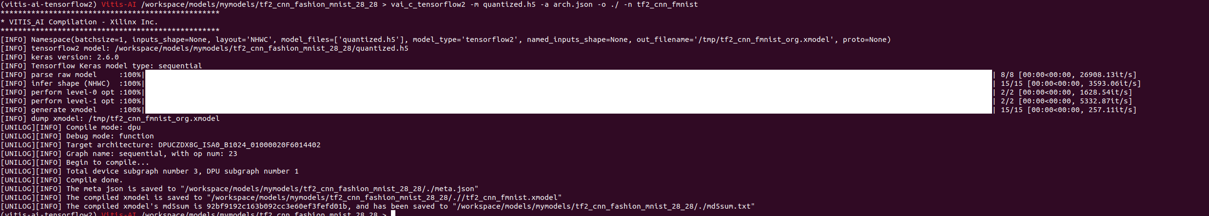
在目录下生成了tf2_cnn_fmnist.xmodel

Inference

首先在设备上需要安装VART相关工具,安装脚本在VitisAI仓库的setup/mpsoc/VART中,将该目录下的target_vart_setup.sh拷贝到设备上运行

编写推理Python程序

1
2
3
4
5
6
7
8
9
10
11
12
13
14
15
16
17
18
19
20
21
22
23
24
25
26
27
28
29
30
31
32
33
34
35
36
37
38
39
40
41
42
43
44
45
46
47
48
49
50
51
52
53
54
55
56
57
58
59
60
61
62
63
64
65
66
import sys
import time
import cv2
import xir
import vart
import math
import numpy as np

def get_graph_from_model(path):
graph = xir.Graph.deserialize(path)
root = graph.get_root_subgraph()
if root.is_leaf:
return []
cs = root.toposort_child_subgraph()
return [
c for c in cs
if cc.has_attr("device") and c.get_attr("device").upper() == "DPU"
]

def image_preprocess(path, input_scale):
print('input_scale:{}'.format(input_scale))
image = cv2.imread(path, 0)
image = image / 2
image = image.astype(np.int8)
return image

def model_run(runner, img):
input_tensors = runner.get_input_tensors()
output_tensors = runner.get_output_tensors()
print('input tensor type:{}'.format(input_tensors))
input_ndim = tuple(input_tensors[0].dims)
print('input_ndim:{}'.format(input_ndim))
output_ndim = tuple(output_tensors[0].dims)
print('output_ndim:{}'.format(output_ndim))
input_data = [np.empty(input_ndim, dtype=np.int8, order="C")]
output_data = [np.empty(output_ndim, dtype=np.int8, order="C")]
print('image shape:{}'.format(img.shape))
#input_data[0] = img.reshape(input_ndim[1:])
job_id = runner.execute_async(img.reshape((1,28,28,1)), output_data)
runner.wait(job_id)
print(output_data)
return np.argmax(output_data[0])

def main(argv):
image_path = argv[1]
model_path = argv[2]
print('image path:{}\nmodel path:{}'.format(
image_path, model_path))

graph = get_graph_from_model(model_path)
dpu_runner = vart.Runner.create_runner(graph[0], "run")
input_fixpos = dpu_runner.get_input_tensors()[0].get_attr("fix_point")
input_scale = 2**input_fixpos
image_data = image_preprocess(image_path, input_scale)
print('image shape:{}'.format(image_data.shape))
print('{}'.format(image_data.reshape((28,28,1))))
time_start = time.time()
pred = model_run(dpu_runner, image_data)
print('pred:{}'.format(pred))
time_end = time.time()

timetotal = time_end - time_start
print('total time:{}'.format(timetotal))

if __name__ == "__main__":
main(sys.argv)

将推理程序、编译后的xmodel模型文件以及测试图片拷贝到设备中,运行推理程序,传入测试图片路径和模型文件路径进行推理,会打印出预测结果

推理代码主要使用了VART API,主要步骤为

  • 加载模型并转换为计算图graph
  • 根据计算图生成DPU Runner
  • 加载输入图片预处理,并构建输入输出Tensor,需要注意各Tensor的shape和dtype
  • 输入输出Tensor传入DPU Runner,异步执行,并同步等待结果
  • 输出Tensor转换为期望的预测数据格式